Components in Latent Diffusion models

Date: June 25, 2023 | Estimated reading time: 10 min | Author: Nikhil Salodkar

Generative Modelling

Diffusion

Huggingface

TABLE OF CONTENTS

1.Loading a pipeline with pre-trained models#loading-a-pipeline-with-pre-trained-models
2.Performing simple inference call#performing-simple-inference-call
3.Inference and training mechanism#inference-and-training-mechanism
4.Individual components and their working in detail#individual-components-and-their-working-in-detail
4.1.Variational Autoencoder (VAE)#variational-autoencoder-vae
4.2.Text Encoder#text-encoder
4.3.Denoising UNet#denoising-unet
4.4.Scheduler#scheduler
4.5.Safety Checker and feature extractor#safety-checker-and-feature-extractor
5.Conclusion#conclusion

Generative AI has been predominantly talked about in the media and social media in 2022 and 2023, especially since its capabilities have been shown publicly by OpenAI's DALL-E 2 and Stable Diffusion models by Stability AI. The impressive capability to generate beautiful looking images like in the figure below has mesmerised us on the innovative potential of Deep Learning models and AI in general. Being Data Scientists, our curiosity extends beyond just using the models and playing around with it. Understanding these models in detail will help us to appreciate properly the power of these models, how might we improve upon them, what are their limitations, and make informed use of them.

Thus, in this blogpost we will go a little bit deeper into understanding such models and their components. We will especially look into Stable diffusion model open-sourced by StabilityAI which can convert textual prompts into images and use the wonderful Huggingface Library "Diffusers" to navigate its working.

Thus, we will look into:

How to load a pre-trained diffusion model and pipeline
Perform a simple inference using the pipeline
Understand the basic mechanism behind how training and inference in Latent diffusion model works
Check out individual components and models inside this stable diffusion pipeline

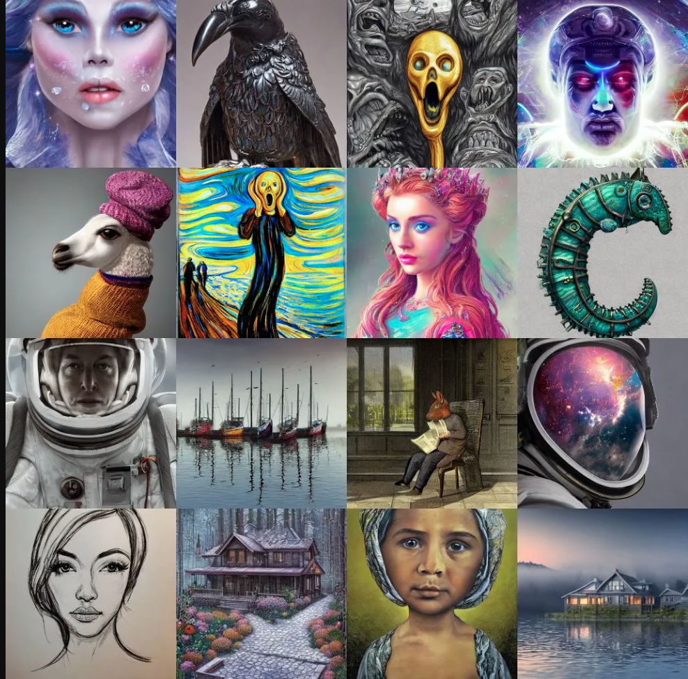
|Samples generated using Generative models | Source: https://creator.nightcafe.studio/stable-diffusion-image-generator |

Setup To try the code snippets on your own, you can either use colab or your own environment but will need to prepare your system to run PyTorch code with the Huggingface Diffusers library. The installation instructions are provided here.

Loading a pipeline with pre-trained models

In huggingface Diffusers library pipeline refers to a class which has methods to load all the components required to run inference on that particular diffusion model. In the below snippet, we are loading stable-diffusion-2-1 pipeline from stabilityai which will download the models if not already downloaded and cached.

from diffusers import StableDiffusionPipeline
repo_id = "stabilityai/stable-diffusion-2-1"
pipe = StableDiffusionPipeline.from_pretrained(repo_id, torch_dtype=torch.float16)

We're loading a variant model having half precision weights only to save memory and time when working with these models. If we pipe.config we get the output:

FrozenDict([('vae', ('diffusers', 'AutoencoderKL')),
            ('text_encoder', ('transformers', 'CLIPTextModel')),
            ('tokenizer', ('transformers', 'CLIPTokenizer')),
            ('unet', ('diffusers', 'UNet2DConditionModel')),
            ('scheduler', ('diffusers', 'DDIMScheduler')),
            ('safety_checker', (None, None)),
            ('feature_extractor', ('transformers', 'CLIPImageProcessor')),
            ('requires_safety_checker', False)])

As we can see, the pipeline loaded many components. Each component fulfills a particular purpose.

VAE : Variational Auto encoder, used to compress the input images into lower dimensional latents which are then in turn used for training the model to make diffusion training faster. Its Encoder is used only during training, and decoder is used during the final step of inference (converting the final denoised image latents to image)
Text Encoder : Transformer model used to convert input text into embeddings which guide what kind of image to be generated.
Tokenizer : Tokenizer for Text Encoder
Unet: The Unet model which in this case is a 2D conditional model to support image inputs to be used to predict the noise which was added to the image at a particular step.
Scheduler : It has logic to determine what, how and for how many steps noise should be added and predicted noise should be removed. There are many different schedulers existing currently, some more efficient than others.
Safety checker : In this particular case, by default, no safety_checker was initialized but in general it refers to a model which, given image features from feature_extractor, returns whether the image features are NSFW or not.

We will look into each component in more detail later.

If we run pipe.to('cuda'), we get the output showcasing all the different components that've been loaded into the gpu.

StableDiffusionPipeline {
  "_class_name": "StableDiffusionPipeline",
  "_diffusers_version": "0.14.0",
  "feature_extractor": [
    "transformers",
    "CLIPImageProcessor"
  ],
  "requires_safety_checker": false,
  "safety_checker": [
    null,
    null
  ],
  "scheduler": [
    "diffusers",
    "DDIMScheduler"
  ],
  "text_encoder": [
    "transformers",
    "CLIPTextModel"
  ],
  "tokenizer": [
    "transformers",
    "CLIPTokenizer"
  ],
  "unet": [
    "diffusers",
    "UNet2DConditionModel"
  ],
  "vae": [
    "diffusers",
    "AutoencoderKL"
  ]
}

Performing simple inference call

The pipeline mechanism allows us to generate images using just a few lines of code. Let's generate a single image.

import torch
generator = torch.Generator('cuda').manual_seed(5)
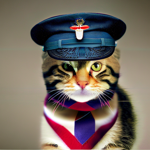
prompt = 'A cute cat wearing a military cap'
%time image = pipe(prompt, generator=generator, width=720, height=720, num_inference_steps=50)

Here, generator was used to seed the image generation process for reproducible results, and we can specify the width and height of the image if required along with num_inference_steps denoising steps to take to generate this image. Keep in mind that the image generation won't work well with low-resolution images like below 512 as the original model was trained using high-resolution images like 768X768 pixels. The output got is the image:

Inference and training mechanism

To understand in detail how the training is done and inference is done, we can refer to the paper High-Resolution Image Synthesis with Latent Diffusion Models. Below is the architecture of the model as mentioned in the paper.

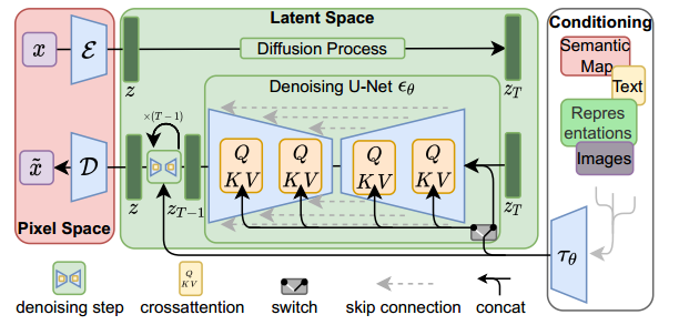
Training and inference architecture |Source: High-Resolution Image Synthesis with Latent Diffusion Models|

As seen in the image above, a latent diffusion model has three main components, A Variational autoencoder with encoder and decoder to convert image to latent space and vice versa as remarked as Pixel Space, A Denoising U-Net model which works in the latent space, and conditioning encoder to help encode conditioning embedding into the Denoising deffuion model.

Inference Phase: The steps during inference phase are:

A random noise is sampled from a distribution which was used during the training phase for timestep T (num_inference_steps)
The condition (in our case text) is tokenized and fed into a text-encoding model to get the text embeddings
The generated random noise can be interpreted as a noisy image Latent.
The noisy image Latent is added as input to the Denoising U-Net for step T-1 along with embedding of condition using a cross-attention mechanism
The Denoising U-Net model predicts the noise present for that step
The predicted noise is subtracted from the noisy image latent from the previous step
The noisy image after subtraction represents a new less noisy image latent
The steps from 4 to 7 are repeated until T reaches zero
At latent embedding generated at step zero is fed through the VAE decoder resulting in the generated image

Training Phase:

Train an autoencoder model or use a good pre-trained one
Train or use pre-trained Conditioning encoder (In stable diffusion case CLIP was used)
Encode an image to lower latent dimension using encoder of VAE
Use the diffusion process to add noise onto the latent image for each diffusion step
Using the noise that was added as ground truth and text embedding with cross-attention as output train the De-noising diffusion model to predict added noise correctly
Repeat from step 3 to step 5 until convergence or generated images start looking adequate when image latent embeddings are decoded back to pixelated images

Individual components and their working in detail

Now that we know the gist of different components used in the stable diffusion pipeline and how the inference and training is done. Let's take a closer look into its components.

Variational Autoencoder (VAE)

The VAE has both encoder and decoder, encoder converting data from image space to lower dimensional latent embedding, and decoder converting lower dimensional latent embedding of image back to image space. The encoder is only used during the training stage when input images are required to be fed to the diffusion model, while during the inference stage (of text to image) only decoder is required to generate images as only text input is given which is not handled by the VAE encoder. Let's try to use the vae encoder and decoder on the cute cat image generated and see if the VAE can be used as a standalone component.

from torchvision.transforms import Compose, ToTensor, Normalize
# transform to convert pil image to normalized tensor
transforms = Compose([ToTensor(), Normalize([0.5], [0.5])])
input_image = transforms(image)
input_image = input_image.unsqueeze(dim=0)
cat_image = input_image.to('cuda')
  cat_image = cat_image.to(torch.float16)
  with torch.no_grad():
      encoded_output = pipe.vae.encode(cat_image).latent_dist.sample()
      print(encoded_output.shape)

The encoded image embedding shape is:

torch.Size([1, 4, 64, 64])

which is very less compared to the original image in pixel space. And this is the encoded_image embedding that is worked upon by the UNET, making the Latent diffusion process much faster.

Now let's try to get back the encoded_output back to pixel space using the decoder and see if we get the same input image.

def numpy_to_pil(images):
        """
        Convert a numpy image or a batch of images to a PIL image.
        """
        if images.ndim == 3:
            images = images[None, ...]
        images = (images * 255).round().astype("uint8")
        if images.shape[-1] == 1:
            # special case for grayscale (single channel) images
            pil_images = [Image.fromarray(image.squeeze(), mode="L") for image in images]
        else:
            pil_images = [Image.fromarray(image) for image in images]
        return pil_images
        
 with torch.no_grad():
        generated_image = pipe.vae.decode(encoded_output).sample
    print(generated_image.shape)
    # code to denormalize the generated image
    generated_image = (generated_image / 2 + 0.5).clamp(0, 1)
    generated_image = generated_image.cpu().permute(0, 2, 3, 1).float().numpy()
    decoded_image = numpy_to_pil(generated_image)
    decoded_image[0].show()

We get the generated image tensor back as torch.Size([1, 3, 512, 512]) and get the almost exact looking image as shown below even though this is a newly generated image with slightly different tensor values.

In this way, we know that the variational autoencoder as an individual component works very well. Let's see what the architecture of the whole VAE looks like by running the command:

from torchinfo import summary
summary(pipe.vae, input_data=input_image, col_names=['input_size', 'output_size', 'num_params'], depth=4)

=============================================================================================================================
Layer (type:depth-idx)                             Input Shape               Output Shape              Param #
=============================================================================================================================
AutoencoderKL                                      [1, 3, 512, 512]          [1, 3, 512, 512]          --
├─Encoder: 1-1                                     [1, 3, 512, 512]          [1, 8, 64, 64]            --
│    └─Conv2d: 2-1                                 [1, 3, 512, 512]          [1, 128, 512, 512]        3,584
│    └─ModuleList: 2-2                             --                        --                        --
│    │    └─DownEncoderBlock2D: 3-1                [1, 128, 512, 512]        [1, 128, 256, 256]        --
│    │    │    └─ModuleList: 4-1                   --                        --                        591,360
│    │    │    └─ModuleList: 4-2                   --                        --                        147,584
│    │    └─DownEncoderBlock2D: 3-2                [1, 128, 256, 256]        [1, 256, 128, 128]        --
│    │    │    └─ModuleList: 4-3                   --                        --                        2,100,224
│    │    │    └─ModuleList: 4-4                   --                        --                        590,080
│    │    └─DownEncoderBlock2D: 3-3                [1, 256, 128, 128]        [1, 512, 64, 64]          --
│    │    │    └─ModuleList: 4-5                   --                        --                        8,394,752
│    │    │    └─ModuleList: 4-6                   --                        --                        2,359,808
│    │    └─DownEncoderBlock2D: 3-4                [1, 512, 64, 64]          [1, 512, 64, 64]          --
│    │    │    └─ModuleList: 4-7                   --                        --                        9,443,328
│    └─UNetMidBlock2D: 2-3                         [1, 512, 64, 64]          [1, 512, 64, 64]          --
│    │    └─ModuleList: 3-7                        --                        --                        (recursive)
│    │    │    └─ResnetBlock2D: 4-8                [1, 512, 64, 64]          [1, 512, 64, 64]          4,721,664
│    │    └─ModuleList: 3-6                        --                        --                        --
│    │    │    └─AttentionBlock: 4-9               [1, 512, 64, 64]          [1, 512, 64, 64]          1,051,648
│    │    └─ModuleList: 3-7                        --                        --                        (recursive)
│    │    │    └─ResnetBlock2D: 4-10               [1, 512, 64, 64]          [1, 512, 64, 64]          4,721,664
│    └─GroupNorm: 2-4                              [1, 512, 64, 64]          [1, 512, 64, 64]          1,024
│    └─SiLU: 2-5                                   [1, 512, 64, 64]          [1, 512, 64, 64]          --
│    └─Conv2d: 2-6                                 [1, 512, 64, 64]          [1, 8, 64, 64]            36,872
├─Conv2d: 1-2                                      [1, 8, 64, 64]            [1, 8, 64, 64]            72
├─Conv2d: 1-3                                      [1, 4, 64, 64]            [1, 4, 64, 64]            20
├─Decoder: 1-4                                     [1, 4, 64, 64]            [1, 3, 512, 512]          --
│    └─Conv2d: 2-7                                 [1, 4, 64, 64]            [1, 512, 64, 64]          18,944
│    └─UNetMidBlock2D: 2-8                         [1, 512, 64, 64]          [1, 512, 64, 64]          --
│    │    └─ModuleList: 3-10                       --                        --                        (recursive)
│    │    │    └─ResnetBlock2D: 4-11               [1, 512, 64, 64]          [1, 512, 64, 64]          4,721,664
│    │    └─ModuleList: 3-9                        --                        --                        --
│    │    │    └─AttentionBlock: 4-12              [1, 512, 64, 64]          [1, 512, 64, 64]          1,051,648
│    │    └─ModuleList: 3-10                       --                        --                        (recursive)
│    │    │    └─ResnetBlock2D: 4-13               [1, 512, 64, 64]          [1, 512, 64, 64]          4,721,664
│    └─ModuleList: 2-9                             --                        --                        --
│    │    └─UpDecoderBlock2D: 3-11                 [1, 512, 64, 64]          [1, 512, 128, 128]        --
│    │    │    └─ModuleList: 4-14                  --                        --                        14,164,992
│    │    │    └─ModuleList: 4-15                  --                        --                        2,359,808
│    │    └─UpDecoderBlock2D: 3-12                 [1, 512, 128, 128]        [1, 512, 256, 256]        --
│    │    │    └─ModuleList: 4-16                  --                        --                        14,164,992
│    │    │    └─ModuleList: 4-17                  --                        --                        2,359,808
│    │    └─UpDecoderBlock2D: 3-13                 [1, 512, 256, 256]        [1, 256, 512, 512]        --
│    │    │    └─ModuleList: 4-18                  --                        --                        4,265,216
│    │    │    └─ModuleList: 4-19                  --                        --                        590,080
│    │    └─UpDecoderBlock2D: 3-14                 [1, 256, 512, 512]        [1, 128, 512, 512]        --
│    │    │    └─ModuleList: 4-20                  --                        --                        1,067,648
│    └─GroupNorm: 2-10                             [1, 128, 512, 512]        [1, 128, 512, 512]        256
│    └─SiLU: 2-11                                  [1, 128, 512, 512]        [1, 128, 512, 512]        --
│    └─Conv2d: 2-12                                [1, 128, 512, 512]        [1, 3, 512, 512]          3,459
=============================================================================================================================
Total params: 83,653,863
Trainable params: 83,653,863
Non-trainable params: 0
Total mult-adds (T): 1.77
=============================================================================================================================
Input size (MB): 1.57
Forward/backward pass size (MB): 6320.10
Params size (MB): 167.31
Estimated Total Size (MB): 6488.98
=============================================================================================================================

As you can see from the architecture summary, the encoder and decoder of VAE is composed of downsampling and upsampling blocks having a total of more than 83 million parameters.

Text Encoder

In this stable diffusion model CLIP is the text encoder model which is being used to convert input text into embeddings which are in turn fed into the Denoising UNet through cross attention mechanism. A pre-trained Text Encoder model is required before it can be used for inference or even before training the Denoising Unet.

Let's see how to use this text encoder as an individual component.

prompt = 'A cute cat wearing a military cap'
# first use the tokenizer to tokenize the text
tokenized_input = pipe.tokenizer(prompt,
                                padding="max_length",
                max_length=pipe.tokenizer.model_max_length,
                truncation=True,
                return_tensors="pt",)
# Then feed the tokenized input into the pre-trained text encoder
device='cuda'
with torch.no_grad():
    prompt_embeds = pipe.text_encoder(tokenized_input.input_ids.to(device),
                attention_mask=tokenized_input.attention_mask.to(device))
print(prompt_embeds)
print(prompt_embeds[0].shape

We get the output showing that the model returns the last hidden state with embedding shape (77, 1024) which will be used as input to provide condition to the Denoising UNet model. The dimensions here show that this particular model can take max number of 77 input tokens and each token has embedding of size 1024.

BaseModelOutputWithPooling(last_hidden_state=tensor([[[-0.3132, -0.4478, -0.0083,  ...,  0.2544, -0.0328, -0.2959],
         [ 0.1989, -1.6963, -0.8945,  ...,  0.4661, -0.0971, -2.1465],
         [ 0.2866, -1.2178,  0.7192,  ...,  0.2888, -1.3584, -1.8545],
         ...,
         [-0.2416, -0.3135, -0.0061,  ...,  0.1088,  0.2859, -0.1702],
         [-0.2378, -0.3020, -0.0081,  ...,  0.1044,  0.3022, -0.1558],
         [-0.0176,  0.0358,  0.6011,  ...,  1.1230,  0.6147,  1.1191]]],
       device='cuda:0', dtype=torch.float16), pooler_output=tensor([[-0.1115, -0.2644,  0.8809,  ...,  1.1650,  0.7417,  1.3916]],
       device='cuda:0', dtype=torch.float16), hidden_states=None, attentions=None)
torch.Size([1, 77, 1024])

The architecture summary of this text encoder looks like this,

summary(pipe.text_encoder, input_data=[tokenized_input.input_ids.to(device), tokenized_input.attention_mask.to(device)],
 col_names=['input_size', 'output_size', 'num_params'])

==================================================================================================================================Layer (type:depth-idx)                                  Input Shape               Output Shape              Param #
==================================================================================================================================
CLIPTextModel                                           [1, 77]                   [1, 1024]                 --
├─CLIPTextTransformer: 1-1                              --                        [1, 1024]                 --
│    └─CLIPTextEmbeddings: 2-1                          --                        [1, 77, 1024]             --
│    │    └─Embedding: 3-1                              [1, 77]                   [1, 77, 1024]             50,593,792
│    │    └─Embedding: 3-2                              [1, 77]                   [1, 77, 1024]             78,848
│    └─CLIPEncoder: 2-2                                 --                        [1, 77, 1024]             --
│    │    └─ModuleList: 3-3                             --                        --                        289,713,152
│    └─LayerNorm: 2-3                                   [1, 77, 1024]             [1, 77, 1024]             2,048
==================================================================================================================================
Total params: 340,387,840
Trainable params: 340,387,840
Non-trainable params: 0
Total mult-adds (M): 340.39
==================================================================================================================================
Input size (MB): 0.00
Forward/backward pass size (MB): 80.74
Params size (MB): 680.78
Estimated Total Size (MB): 761.52
==================================================================================================================================

having 340 million parameters.

Denoising UNet

The Denoising UNet is the main component of the whole Latent diffusion model because this model is the one which actually is able to iteratively convert a random noise following a particular distribution to a good image embedding by predicting the noise which is present in the input which can then be subtracted from the original noisy image to get a less noisy image.

The UNet forward method takes three mandatory input arguments-The encoded noisy image, the encoded text prompt for condition, and the denoising step for which prediction needs to be done.

Let's try this out for 4th step as an example:

timestep=4
with torch.no_grad():
    unet_output = pipe.unet(encoded_output, timestep, prompt_embeds[0])
    print(unet_output.sample.shape)

We get the output

torch.Size([1, 4, 64, 64])

which is exactly the size of encoded noisy image. We can infer the same by looking at the UNet architecture summary.

summary(pipe.unet, input_data=[encoded_output, 4, prompt_embeds[0]], col_names=['output_size', 'num_params'])

===================================================================================================================Layer (type:depth-idx)                                            Output Shape              Param #
===================================================================================================================
UNet2DConditionModel                                              [1, 4, 64, 64]            --
├─Timesteps: 1-1                                                  [1, 320]                  --
├─TimestepEmbedding: 1-2                                          [1, 1280]                 --
│    └─Linear: 2-1                                                [1, 1280]                 410,880
│    └─SiLU: 2-2                                                  [1, 1280]                 --
│    └─Linear: 2-3                                                [1, 1280]                 1,639,680
├─Conv2d: 1-3                                                     [1, 320, 64, 64]          11,840
├─ModuleList: 1-4                                                 --                        --
│    └─CrossAttnDownBlock2D: 2-4                                  [1, 320, 32, 32]          --
│    │    └─ModuleList: 3-3                                       --                        (recursive)
│    │    └─ModuleList: 3-4                                       --                        (recursive)
│    │    └─ModuleList: 3-3                                       --                        (recursive)
│    │    └─ModuleList: 3-4                                       --                        (recursive)
│    │    └─ModuleList: 3-5                                       --                        921,920
│    └─CrossAttnDownBlock2D: 2-5                                  [1, 640, 16, 16]          --
│    │    └─ModuleList: 3-8                                       --                        (recursive)
│    │    └─ModuleList: 3-9                                       --                        (recursive)
│    │    └─ModuleList: 3-8                                       --                        (recursive)
│    │    └─ModuleList: 3-9                                       --                        (recursive)
│    │    └─ModuleList: 3-10                                      --                        3,687,040
│    └─CrossAttnDownBlock2D: 2-6                                  [1, 1280, 8, 8]           --
│    │    └─ModuleList: 3-13                                      --                        (recursive)
│    │    └─ModuleList: 3-14                                      --                        (recursive)
│    │    └─ModuleList: 3-13                                      --                        (recursive)
│    │    └─ModuleList: 3-14                                      --                        (recursive)
│    │    └─ModuleList: 3-15                                      --                        14,746,880
│    └─DownBlock2D: 2-7                                           [1, 1280, 8, 8]           --
│    │    └─ModuleList: 3-16                                      --                        62,277,120
├─UNetMidBlock2DCrossAttn: 1-5                                    [1, 1280, 8, 8]           --
│    └─ModuleList: 2-10                                           --                        (recursive)
│    │    └─ResnetBlock2D: 3-17                                   [1, 1280, 8, 8]           31,138,560
│    └─ModuleList: 2-9                                            --                        --
│    │    └─Transformer2DModel: 3-18                              [1, 1280, 8, 8]           35,416,320
│    └─ModuleList: 2-10                                           --                        (recursive)
│    │    └─ResnetBlock2D: 3-19                                   [1, 1280, 8, 8]           31,138,560
├─ModuleList: 1-6                                                 --                        --
│    └─UpBlock2D: 2-11                                            [1, 1280, 16, 16]         --
│    │    └─ModuleList: 3-20                                      --                        147,494,400
│    │    └─ModuleList: 3-21                                      --                        14,746,880
│    └─CrossAttnUpBlock2D: 2-12                                   [1, 1280, 32, 32]         --
│    │    └─ModuleList: 3-26                                      --                        (recursive)
│    │    └─ModuleList: 3-27                                      --                        (recursive)
│    │    └─ModuleList: 3-26                                      --                        (recursive)
│    │    └─ModuleList: 3-27                                      --                        (recursive)
│    │    └─ModuleList: 3-26                                      --                        (recursive)
│    │    └─ModuleList: 3-27                                      --                        (recursive)
│    │    └─ModuleList: 3-28                                      --                        14,746,880
│    └─CrossAttnUpBlock2D: 2-13                                   [1, 640, 64, 64]          --
│    │    └─ModuleList: 3-33                                      --                        (recursive)
│    │    └─ModuleList: 3-34                                      --                        (recursive)
│    │    └─ModuleList: 3-33                                      --                        (recursive)
│    │    └─ModuleList: 3-34                                      --                        (recursive)
│    │    └─ModuleList: 3-33                                      --                        (recursive)
│    │    └─ModuleList: 3-34                                      --                        (recursive)
│    │    └─ModuleList: 3-35                                      --                        3,687,040
│    └─CrossAttnUpBlock2D: 2-14                                   [1, 320, 64, 64]          --
│    │    └─ModuleList: 3-40                                      --                        (recursive)
│    │    └─ModuleList: 3-41                                      --                        (recursive)
│    │    └─ModuleList: 3-40                                      --                        (recursive)
│    │    └─ModuleList: 3-41                                      --                        (recursive)
│    │    └─ModuleList: 3-40                                      --                        (recursive)
│    │    └─ModuleList: 3-41                                      --                        (recursive)
├─GroupNorm: 1-7                                                  [1, 320, 64, 64]          640
├─SiLU: 1-8                                                       [1, 320, 64, 64]          --
├─Conv2d: 1-9                                                     [1, 4, 64, 64]            11,524
===================================================================================================================
Total params: 865,910,724
Trainable params: 865,910,724
Non-trainable params: 0
Total mult-adds (G): 209.52
===================================================================================================================
Input size (MB): 0.19
Forward/backward pass size (MB): 1265.48
Params size (MB): 1731.82
Estimated Total Size (MB): 2997.49
===================================================================================================================

As we can see above, the UNet model has around 865 million parameters and has cross attention blocks which integrate the text embeddings into the noisy image embeddings.

Scheduler

The last important component to look at is the scheduler. It does not have any parameters just like the text_encoder, but is essential because it handles all the logic around noise management like in what way to add noise to image embedding for a particular scheduling step, how to remove noise using the predicted noise by UNet, and handling some hyperparameters related to scheduling algorithm. If we print print(pipe.scheduler) we get the output

DDIMScheduler {
  "_class_name": "DDIMScheduler",
  "_diffusers_version": "0.14.0",
  "beta_end": 0.012,
  "beta_schedule": "scaled_linear",
  "beta_start": 0.00085,
  "clip_sample": false,
  "num_train_timesteps": 1000,
  "prediction_type": "v_prediction",
  "set_alpha_to_one": false,
  "skip_prk_steps": true,
  "steps_offset": 1,
  "trained_betas": null
}

which shows that we're using DDIMScheduler with its version and different default hyperparameters. It has methods such as set_timesteps(to set the max timesteps for inference) and step(predict the noise at the previous time step) to facilitate easier training and inference operations. To get more information around different schedulers and their usage, check out Huggingface diffusers documentation.

Safety Checker and feature extractor

Safety checker a model which checks if the NSFW content is being generated and if so, flags it with a warning and generates a blank image if the "requires_safety_checker" is set to True. "feature_extractor" is used to extract features from generated image to be fed to the safety_checker model.

Conclusion

In this blogpost, we saw how different components work in tandem in a Latent diffusion model using the transformer's Diffusers library. For complex models such as diffusion models, it is always a good practice to check out how individual components work to understand the working clearly.

Home

Consultation Services

Development Services

About